Notes on SUMO Unbiased Estimation of Log-Partition Function

(2020/02/11)

In this note, I'll implement the Stochastically Unbiased Marginalization Objective (SUMO) to estimate the log-partition function of an energy funtion.

Estimation of log-partition function has many important applications in machine learning. Take latent variable models or Bayeisian inference. The log-partition function of the posterior distribution $p(z|x)=\frac{1}{Z}p(x|z)p(z)$ is the log-marginal likelihood of the data $\log Z = \log \int p(x|z)p(z)dz = \log p(x)$.

More generally, let $U(x)$ be some energy function which induces some density function $p(x)=\frac{e^{-U(x)}}{\int e^{-U(x)} dx}$. The common practice is to look at a variational form of the log-partition function,

Plugging in an arbitrary $q$ would normally yield a strict lower bound, which means

for $x_i$ sampled i.i.d. from $q$, would be a biased estimate for $\log Z$. In particular, it would be an underestimation.

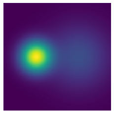
To see this, lets define the energy function $U$ as follows:

It is not hard to see that $U$ is the energy function of a mixture of Gaussian distribution $\frac{1}{2}\mathcal{N}([-2,0], I) + \frac{1}{2}\mathcal{N}([2,0], 4I)$ with a normalizing constant $Z=2\pi\approx6.28$ and $\log Z\approx1.8379$.

def U(x):
  x1 = x[:,0]
  x2 = x[:,1]
  d2 = x2 ** 2
  return - np.log(np.exp(-((x1+2) ** 2 + d2)/2)/2 + np.exp(-((x1-2) ** 2 + d2)/8)/4/2)

To visualize the density corresponding to the energy $p(x)\propto e^{-U(x)}$

xxxxxxxxxx
xx = np.linspace(-5,5,200)
yy = np.linspace(-5,5,200)
X = np.meshgrid(xx,yy)
X = np.concatenate([X[0][:,:,None], X[1][:,:,None]], 2).reshape(-1,2)
unnormalized_density = np.exp(-U(X)).reshape(200,200)
plt.imshow(unnormalized_density)
plt.axis('off')

As a sanity check, lets also visualize the density of the mixture of Gaussians.

xxxxxxxxxx
N1, N2 = mvn([-2,0], 1), mvn([2,0], 4)
density = (np.exp(N1.logpdf(X))/2 + np.exp(N2.logpdf(X))/2).reshape(200,200)
plt.imshow(density)
plt.axis('off')
print(np.allclose(unnormalized_density / density - 2*np.pi, 0))

 True 

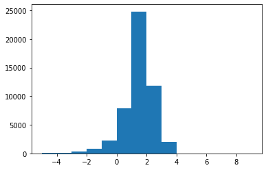
Now if we estimate the log-partition function by estimating the variational lower bound, we get

​x
q = mvn([0,0],5)
​
xs = q.rvs(10000*5)
elbo = - U(xs) - q.logpdf(xs)
plt.hist(elbo, range(-5,10))
print("Estimate:  %.4f  / Ground true:  %.4f" % (elbo.mean(), np.log(2*np.pi)))
print("Empirical variance: %.4f" % elbo.var())

Estimate:  1.4595  / Ground true:  1.8379
Empirical variance: 0.9921

The lower bound can be tightened via [importance sampling):

This bound is tighter for larger $K$ partly due to the concentration of the average inside of the $\log$ function: when the random variable is more deterministic, using a local linear approximation near its mean is more accurate as there's less "mass" outside of some neighborhood of the mean.

Now if we use this new estimator with $K=5$

xxxxxxxxxx
k = 5
xs = q.rvs(10000*k)
elbo = - U(xs) - q.logpdf(xs)
iwlb = elbo.reshape(10000,k)
iwlb = np.log(np.exp(iwlb).mean(1))
plt.hist(iwlb, range(-5,10))
print("Estimate:  %.4f  / Ground true:  %.4f" % (iwlb.mean(), np.log(2*np.pi)))
print("Empirical variance: %.4f" % iwlb.var())

Estimate:  1.7616  / Ground true:  1.8379
Empirical variance: 0.1544

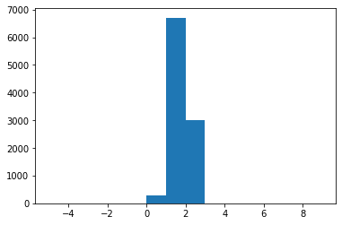
We see that both the bias and variance decrease.

Finally, we use the Stochastically Unbiased Marginalization Objective (SUMO), which uses the Russian Roulette estimator to randomly truncate a telescoping series that converges in expectation to the log partition function. Let $\text{IWAE}_K = \log\left(\frac{1}{K}\sum_{j=1}^K \frac{e^{-U(x_j)}}{q(x_j)}\right)$ be the importance-weighted estimator, and $\Delta_K = \text{IWAE}_{K+1} - \text{IWAE}_K$ be the difference (which can be thought of as some form of correction). The SUMO estimator is defined as

where $K\sim p(K)=\mathbb{P}(\mathcal{K}=K)$. To see why this is an unbiased estimator,

The inner expectation can be further expanded

which shows $\mathbb{E}[\text{SUMO}] = \mathbb{E}[\text{IWAE}_\infty] = \log Z$.

(N.B.) Some care needs to be taken care of for taking the limit. See the paper for more formal derivation.

A choice of $P(K)$ proposed in the paper satisfy $\mathbb{P}(\mathcal{K}\geq K)=\frac{1}{K}$. We can sample such a $K$ easily using the inverse CDF, $K=\lfloor\frac{u}{1-u}\rfloor$ where $u$ is sampled uniformly from the interval $[0,1]$.

Now putting things all together, we can estimate the log-partition using SUMO.

xxxxxxxxxx
count = 0
bs = 10
iwlb = list()
while count <= 1000000:
  u = np.random.rand(1)
  k = np.ceil(u/(1-u)).astype(int)[0]
  xs = q.rvs(bs*(k+1))
  elbo = - U(xs) - q.logpdf(xs)
  iwlb_ = elbo.reshape(bs, k+1)
  iwlb_ = np.log(np.cumsum(np.exp(iwlb_), 1) / np.arange(1,k+2))
  iwlb_ = iwlb_[:,0] + ((iwlb_[:,1:k+1] - iwlb_[:,0:k]) * np.arange(1,k+1)).sum(1)
  count += bs * (k+1)
  iwlb.append(iwlb_)
​
iwlb = np.concatenate(iwlb)
plt.hist(iwlb, range(-5,10))
print("Estimate:  %.4f  / Ground true:  %.4f" % (iwlb.mean(), np.log(2*np.pi)))
print("Empirical variance: %.4f" % iwlb.var())

Estimate:  1.8359  / Ground true:  1.8379
Empirical variance: 4.1794

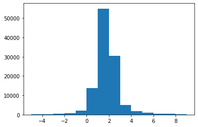
Indeed the empirical average is quite close to the true log-partition of the energy function. However we can also see that the distribution of the estimator is much more spread-out. In fact, it is very heavy-tailed. Note that I did not tune the proposal distribution $q$ based on the ELBO, or IWAE or SUMO. In the paper, the authors propose to tune $q$ to minimize the variance of the $\text{SUMO}$ estimator, which might be an interesting trick to look at next.